※参考<統計ソフトRに入力するコマンド>
統計ソフトRのインストール手順をまとめた記事も作成していますので、よろしければご参考ください。
library(BasketballAnalyzeR)
library(gridExtra)
library(ggplot2)
library(ggrepel)
Tbox2526 <- read.csv(file="Tbox_20260209.csv")
Obox2526 <- read.csv(file="Obox_20260209.csv")
Tadd2526 <- read.csv(file="Tadd_20260209.csv")
fourfactors2526 <- fourfactors(Tbox2526, Obox2526)
Playoff <- Tadd2526$Playoff
fourfactors2526 <- data.frame(fourfactors2526, Playoff)
fourfactors2526
# PACE of NBA teams
ggplot(data=fourfactors2526, aes(x=PACE.Off, y=PACE.Def, color = Playoff, label=Team)) +
geom_point() +
ggrepel::geom_text_repel(aes(label = Team))+
geom_vline(xintercept =mean(fourfactors2526$PACE.Off))+
geom_hline(yintercept =mean(fourfactors2526$PACE.Def))+
labs(title = "PACE (as of 20260209)")+
labs(x = "Pace (Possessions per minute) of the Team") +
labs(y = "Pace (Possessions per minute) of the Opponents")
# Rtg of NBA teams
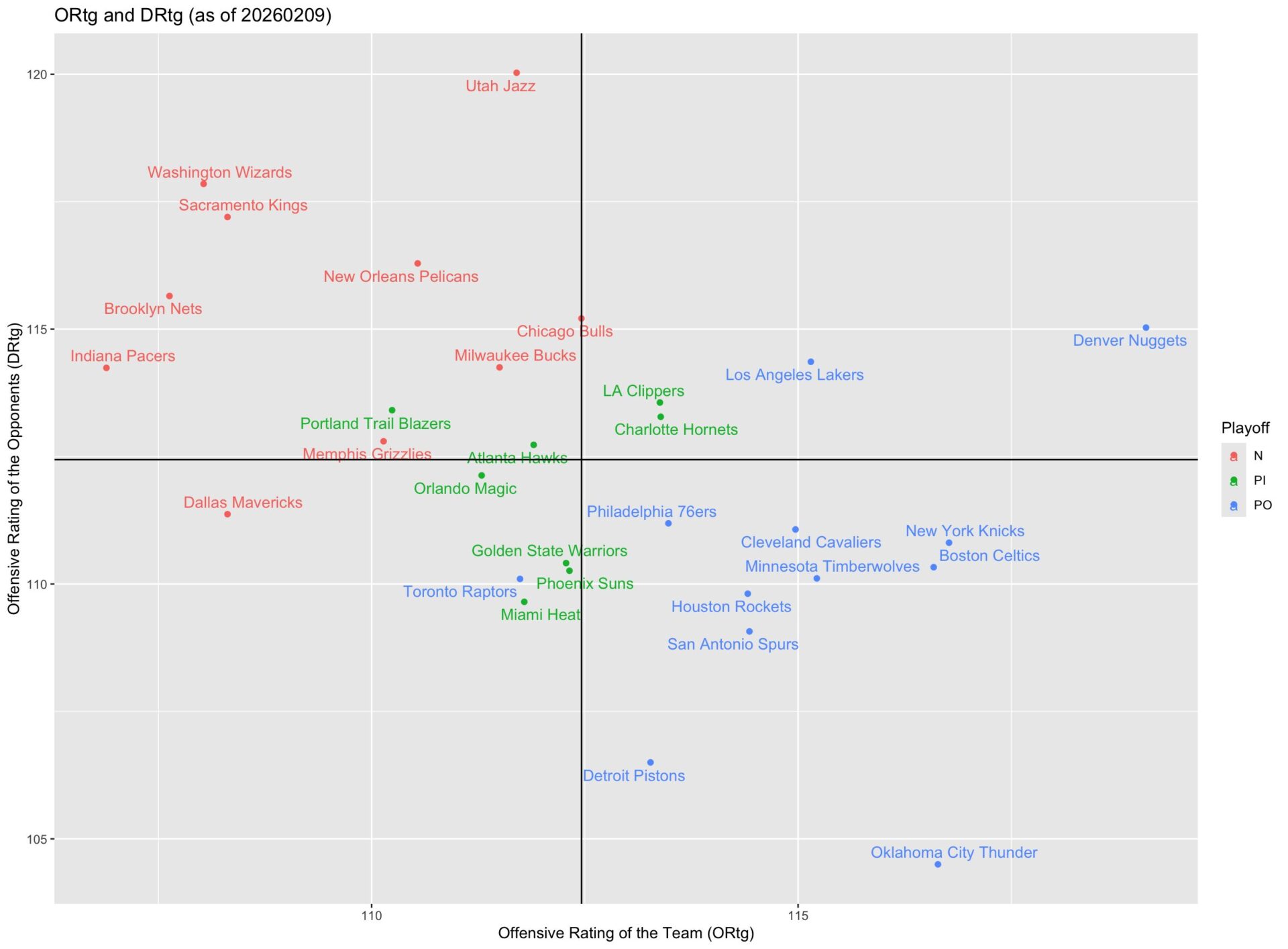
ggplot(data=fourfactors2526, aes(x=ORtg, y=DRtg, color = Playoff, label=Team)) +
geom_point() +
ggrepel::geom_text_repel(aes(label = Team))+
geom_vline(xintercept =mean(fourfactors2526$ORtg))+
geom_hline(yintercept =mean(fourfactors2526$DRtg))+
labs(title = "ORtg and DRtg (as of 20260209)")+
labs(x = "Offensive Rating of the Team (ORtg)") +
labs(y = "Offensive Rating of the Opponents (DRtg)")
# eFG% of NBA teams
ggplot(data=fourfactors2526, aes(x=F1.Off, y=F1.Def, color = Playoff, label=Team)) +
geom_point() +
ggrepel::geom_text_repel(aes(label = Team))+
geom_vline(xintercept =mean(fourfactors2526$F1.Off))+
geom_hline(yintercept =mean(fourfactors2526$F1.Def))+
labs(title = "Factor 1:eFG% (as of 20260209)")+
labs(x = "eFG% (Offense)") +
labs(y = "eFG% (Defense)")
# TO Ratio of NBA teams
ggplot(data=fourfactors2526, aes(x=F2.Off, y=F2.Def, color = Playoff, label=Team)) +
geom_point() +
ggrepel::geom_text_repel(aes(label = Team))+
geom_vline(xintercept =mean(fourfactors2526$F2.Off))+
geom_hline(yintercept =mean(fourfactors2526$F2.Def))+
labs(title = "Factor 2:TO Ratio (as of 20260209)")+
labs(x = "TO Ratio (Offense)") +
labs(y = "TO Ratio (Defense)")
# REB% of NBA teams
ggplot(data=fourfactors2526, aes(x=F3.Off, y=F3.Def, color = Playoff, label=Team)) +
geom_point() +
ggrepel::geom_text_repel(aes(label = Team))+
geom_vline(xintercept =mean(fourfactors2526$F3.Off))+
geom_hline(yintercept =mean(fourfactors2526$F3.Def))+
labs(title = "Factor 3:REB% (as of 20260209)")+
labs(x = "REB% (Offense)") +
labs(y = "REB% (Defense)")
# FT Rate of NBA teams
ggplot(data=fourfactors2526, aes(x=F4.Off, y=F4.Def, color = Playoff, label=Team)) +
geom_point() +
ggrepel::geom_text_repel(aes(label = Team))+
geom_vline(xintercept =mean(fourfactors2526$F4.Off))+
geom_hline(yintercept =mean(fourfactors2526$F4.Def))+
labs(title = "Factor 4:FT Rate (as of 20260209)")+
labs(x = "FT Rate (Offense)") +
labs(y = "FT Rate (Defense)")
# ラベルまとめ表
quadrant_label <- function(x, y, x_mean, y_mean,
ll, lr, ul, ur) {
if (x < x_mean & y < y_mean) return(ll) # 左下
if (x > x_mean & y < y_mean) return(lr) # 右下
if (x < x_mean & y > y_mean) return(ul) # 左上
if (x > x_mean & y > y_mean) return(ur) # 右上
}
# PACE
pace_labels <- list(
ll = "ペースコントロール型",
lr = "ペース主導型",
ul = "ペース受動型",
ur = "多展開型"
)
# Ratings (ORtg × DRtg)
rtg_labels <- list(
ll = "守備優勢型",
lr = "攻守安定型",
ul = "再建段階型",
ur = "攻撃優勢型"
)
# eFG%
efg_labels <- list(
ll = "低効率均衡型",
lr = "シュート優位型",
ul = "効率劣勢型",
ur = "打ち合い型"
)
# TO Ratio
to_labels <- list(
ll = "ロスト抑制型",
lr = "自滅型",
ul = "ポゼッション優位型",
ur = "ロスト多発型"
)
# REB%
reb_labels <- list(
ll = "インサイド劣勢型",
lr = "セカンドチャンス重視型",
ul = "ディフェンスリバウンド重視型",
ur = "インサイド支配型"
)
# FT Rate
ft_labels <- list(
ll = "クリーンゲーム型",
lr = "ファウル活用型",
ul = "フィジカル劣勢型",
ur = "肉弾戦型"
)
df <- fourfactors2526
# 平均値
mx_pace <- mean(df$PACE.Off); my_pace <- mean(df$PACE.Def)
mx_rtg <- mean(df$ORtg); my_rtg <- mean(df$DRtg)
mx_f1 <- mean(df$F1.Off); my_f1 <- mean(df$F1.Def)
mx_f2 <- mean(df$F2.Off); my_f2 <- mean(df$F2.Def)
mx_f3 <- mean(df$F3.Off); my_f3 <- mean(df$F3.Def)
mx_f4 <- mean(df$F4.Off); my_f4 <- mean(df$F4.Def)
# ラベル付け
df$PACE_Label <- mapply(quadrant_label, df$PACE.Off, df$PACE.Def,
MoreArgs = c(mx_pace, my_pace, pace_labels))
df$RTG_Label <- mapply(quadrant_label, df$ORtg, df$DRtg,
MoreArgs = c(mx_rtg, my_rtg, rtg_labels))
df$eFG_Label <- mapply(quadrant_label, df$F1.Off, df$F1.Def,
MoreArgs = c(mx_f1, my_f1, efg_labels))
df$TO_Label <- mapply(quadrant_label, df$F2.Off, df$F2.Def,
MoreArgs = c(mx_f2, my_f2, to_labels))
df$REB_Label <- mapply(quadrant_label, df$F3.Off, df$F3.Def,
MoreArgs = c(mx_f3, my_f3, reb_labels))
df$FT_Label <- mapply(quadrant_label, df$F4.Off, df$F4.Def,
MoreArgs = c(mx_f4, my_f4, ft_labels))
# Team を結合
df_joined <- merge(Tadd2526[, c("Team", "Rank", "Conference", "Division")],
df[, c("Team",
"PACE_Label", "RTG_Label", "eFG_Label",
"TO_Label", "REB_Label", "FT_Label")],
by = "Team",
all.x = TRUE)
team_labels <- df_joined[order(df_joined$Rank), ]
library(readr)
write_excel_csv(team_labels, "team_rank_6labels_20260209_autoJP_withRankConf.csv"